Likert-graphs in R, embedding metadata for easier plotting
October 2, 2013, [MD]
I've been working a lot with questionnaire data in R lately. Some are large MOOC-questionnaires with up to 20,000 respondents, others are in-class surveys with 30-250 respondents, where we have to type or scan in the response sheets. However, once it comes to data cleanup and analysis, there is not much difference between 30 and 20,000 respondents. Here's an example of a section of a recent survey we distributed to around 600 undergraduates in history and religion:
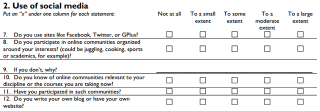
Before beginning to do any kind of statistical tests or modeling, I like to generate graphs of the different questions, both univariate, and split across other variables. Most of the questions are typically likert-type questions, where you have a number of options from "Very unlikely" to "Very likely", or "Not at all" to "To a large extent" -- these are all converted into ordered factors. The questions in the dataframe will then end up like this:
> db[1:5,9:14]
                    X7                   X8   X9               X10        X11        X12
1       To some extent           Not at all <NA>        Not at all       <NA> Not at all
2 To a moderate extent    To a small extent <NA> To a small extent Not at all Not at all
3       To some extent    To a small extent <NA> To a small extent Not at all Not at all
4 To a moderate extent To a moderate extent <NA>        Not at all Not at all Not at all
5    To a small extent To a moderate extent <NA>        Not at all Not at all Not at all
There are many ways of plotting this data, and one of the simplest one would probably be a stacked barchart (taken from statistical-research.com):
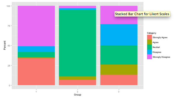
Diverging stacked bar chart
However, a much more intuitive way of presenting the data is a diverging stacked bar chart, where you center around the neutral value (or remove the neutral altogether), with the less-than-neutral values plotted to the left, and the more-than-neutral to the right. At a glance, you can easily compare different questions, or the same question split over another variable.
Initially, I used the likert function in the HH package, which worked, but was not ideal. It was based on Trellis-graphics, instead of GGPlot2, which provides less flexibility in manipulating the graphs afterwards. It also wanted a frequency table, which meant I had to write some functions to transform my data -- not too difficult, but adding in complexity and potential for error (the functions I wrote).
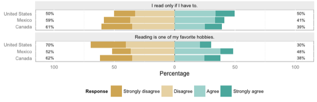
So I was very happy to come across Jason Bryer's likert-package, which works directly on the kind of format I showed above, and outputs beautiful graphs. Here's a truncated example from the documentation, splitting two of the test items on a demographic variable:
require(likert)
data(pisaitems)

##### Item 24: Reading Attitudes
items24 <- pisaitems[,substr(names(pisaitems), 1,5) == 'ST24Q']

items24 <- rename(items24, c(
            ST24Q01="I read only if I have to.",
            ST24Q02="Reading is one of my favorite hobbies.",
            ST24Q03="I like talking about books with other people.",
            ST24Q04="I find it hard to finish books.",
            ST24Q05="I feel happy if I receive a book as a present.",
            ST24Q06="For me, reading is a waste of time.",
            ST24Q07="I enjoy going to a bookstore or a library.",
            ST24Q08="I read only to get information that I need.",
            ST24Q09="I cannot sit still and read for more than a few minutes.",
            ST24Q10="I like to express my opinions about books I have read.",
            ST24Q11="I like to exchange books with my friends."))
l24g <- likert(items24[,1:2], grouping=pisaitems$CNT)
plot(l24g)
Data is data, and code is code
This was very close to what I wanted, but something about the code above struck me as messy. Usually when I'm working on data analysis, I will create a separate script to load in, clean up and prepare the data for analysis. During this work, I take care to not modify the source files at all, and that the processing pipeline can be re-run over the raw input data again generating exactly the same output.
For example, in the above example, I had actually received Excel-files from a number of students who helped me with data entry. Instead of copying and pasting this data into one large Excel-spreadsheet, I read them all into R, combined them and cleaned up ideosyncrasies, preserving the original Excel-files:
ana <- read.xlsx(file="ana.xlsx", 1, stringsAsFactors=FALSE)
chad <- read.xlsx(file="chad.xlsx", 1, stringsAsFactors=FALSE)
dd <- read.xlsx(file="dd.xlsx", 1, stringsAsFactors=FALSE)
db <- rbind(ana, chad, dd)
During this cleanup process, I must refer back to the actual questionnaire and make sure that factors make sense, etc. Once I am done, I save to an RData file, start a new script, load the RData file, and begin the process of exploratory analysis and graphing.
When I'm in the mode of exploring the data, I want my data object to contain all the data that I am working with. To me, both how the questions are grouped, and full question titles, are part of the data. So when we're subsetting the data in the example above...
items24 <- pisaitems[,substr(names(pisaitems), 1,5) == 'ST24Q']
...we're actually accessing a semantically logical subset of the data. At least in this case, all the questions of this section had ST24Q... as part of their names, but in my case, I don't even have that.
Even worse is the need to rename the question columns, to have the full questions (or titles) show up in the resulting plot. This is pure information, which should be attached to the object, and follow it around -- instead it's plunked in the middle of a data analysis script. If I end up extracting another group of questions later, I'll have to rename them again. And because these titles typically contain spaces and punctuation, we can't just rename all the columns and work with them like that.
Using attributes to store the metadata
I was trying to figure out a way of storing these attributes as part of the dataframe, and came across the concept of attributes. Any object in R can store an unlimited number of named attributes (ie. a whole dataframe can have attributes, but also the individual columns in the dataframe). The usage is simple,
attr(x, which, exact = FALSE)
attr(x, which) <- value
So for example, in the example above, I could set the names like this:
attr(items24$ST24Q01, "full.name") <- "I read only if I have to."
We could also store the various groupings directly in the dataframe, like this:
attr(items24, "likert.groups") <- list("Question 24" = c("ST24Q01","ST24Q02","ST24Q03"))
These attributes will now follow the objects around, and be saved and loaded from the RData file. However, it's all a bit useless, unless our tools are aware of this metadata.
Making Likert() aware of the metadata
I began opening up the Likert package, and seeing if I could insert support for this metadata. After a bit of fumbling, it turned out to be surprisingly easy. Here's all the code that was required to make it pick up metadata, if present, and carry on as usual if not (from likert.R):
# pull in long names from attributes, if exist
for (n in names(items)) {
  if (!is.null(attr(items[[n]], "fullname"))) {
    names(items)[names(items) == n] <- attr(items[[n]], "fullname")
    }
}
There was of course also some code to enable using the groups, segmenting by the groups if plotting the whole data set, etc. All in all, I ended up with a pull request with 115 new lines, although 40 of those are just documentation.
Pulling it all together
So with this new functionality, I was able to define the names and groups in the script where I process the data, using a simple helper function to set the attributes:
db <- likert_add_fullnames(db, c(
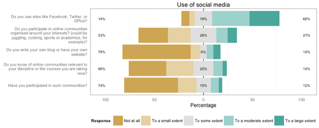
"X7"="Do you use sites like Facebook, Twitter, or GPlus?",
"X8"="Do you participate in online communities organised around your interests?
(could be juggling, cooking, sports or academics, for example)?",
"X10"="Do you know of online communities relevant to your discipline or the
courses you are taking now?"))
...
This goes on for all 42 questions. I then specify the groups of questions:
groups <- list(
  "Use of social media"=c("X7","X8","X10","X11","X12"),
  "Social learning"=c("X13","X14","X15","X16","X17","X18","X19","X20"),
  "Connection with other students"=c("X21","X22","X23","X24","X25"))

db <- likert_store_groups(db, groups)
And that's it. I save the RData file, load it up in my processing script, and I can now do things like...
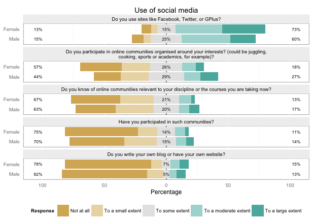
plot_likert_groups(db, groups="Use of social media")
...to plot a simple overview of the first group of variables, with a nice header:
Or I can easily split this on another variable, like gender:
plot_likert_groups(db, groups="Use of social media", grouping=db$gender)
The metadata carries through even if I just want to plot a few variables, not the whole group:
plot(likert(db[,c("X21","X22")], grouping=db$gender))
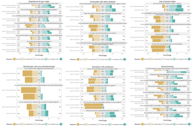
And I can even plot the entire dataset. Here I split the students into two groups, depending on their response to the question "To what extent do you learn from your peers, and not only from the teachers?", and plot every single question, nicely offset per group.
db$learnfrompeers <- ifelse(as.numeric(db$X13) > 3,
  "Learn from peers",
  "Learn only from teachers")

plot_likert_groups(db, all=T, grouping=db$learnfrompeers)
Works for me...
So this all works great, and I'm very happy. I've submitted a pull-request which has been dormant for a month, but on the other hand, I never expected this to be accepted right away. There are many possible ways of doing this, and I am a complete beginner at R programming, I'm sure it could be rewritten in a much cleaner way.
However, fundamentally, this is still a hack. No other function is aware of this metadata, even a simple table to get a frequency table, will not use the full question names. And the attributes on the dataframe are lost upon subsetting. After "reinventing the wheel" with my attribute hack, I realized that the HMisc package actually has a label function which implements the same idea, but also does some magic to make sure the labels are not lost upon subsetting. However, I didn't want to suggest a dependency from Likert upon HMisc, and again, the problem of other functions not knowing about it is still unsolved.
Richer datasets in the open data world?
I'm personally very curious about whether this is something that could be solved at a language level for Julia (which I've been playing with lately), given that they already have support for Units. I'm also interested in how this data could be stored independent of language or tool -- I might want to share my dataset with someone using Python or STATA, and it would be great if these annotations could follow.
I think this is particularly important for the open data movement, which has so far seemed to push for mainly CSV-files. This is much better than PDFs, but there is a lot of information lost, whether all those factors you spent time cleaning up, or annotation, etc.
In fact, when I use the R package WDI to grab the number of journal publications per country from the World Development Indicators like this:
 db<-WDI(country="all", indicator="IP.JRN.ARTC.SC")
> head(db)
  iso2c    country IP.JRN.ARTC.SC year
1    1A Arab World             NA 2011
2    1A Arab World             NA 2010
3    1A Arab World         6578.4 2009
4    1A Arab World         6099.3 2008
5    1A Arab World         5647.7 2007
6    1A Arab World         5247.7 2006
I find it amazing that it's so easy to get access to an open dataset in R, and begin analyzing it... But I wish not only the cryptic indicator was annotated with the full name of the indicator (and explanation), but I would even love for every single number to be annotated. Tell me exactly how you calculated that Afghanistan had 11,700 articles in 2009 (I'm assuming these are in thousands) articles - which data sources that number is compiled from, the margin of error, etc. Only in that way can open data sources become really powerful.
> db[db$country=="Afghanistan",]
    iso2c     country IP.JRN.ARTC.SC year
267    AF Afghanistan             NA 2011
268    AF Afghanistan             NA 2010
269    AF Afghanistan           11.7 2009
270    AF Afghanistan            6.6 2008
271    AF Afghanistan            3.8 2007
272    AF Afghanistan            4.0 2006
273    AF Afghanistan            3.9 2005
Perhaps something like HDF5 is a solution (although it worried me when I tried writing a 180MB dataframe to HDF5, and it ended up being 460 MB), or maybe something like Linked CSV. Either way, I'd love to hear from people interested in discussing this.
Stian Håklev October 2, 2013 Toronto, Canada comments powered by Disqus